Optimization Techniques in Scientific Computing (Part II)

• Introduction and recap
• The first implementation
• Optimization ideas
• Parallelism
  • Core-level
  • Node-level
  • Cluster-level
  • Key consideration

Introduction and recap

In my previous blog, I introduced some straightforward yet valuable optimization techniques. While these techniques are generally suitable for relatively simple problems, such as the example presented in my previous blog, they may prove inadequate when dealing with more complex and realistic issues. Specifically, in the previous example, my objective was to simulate a single-molecule microscope image. However, people frequently need to process multiple independent images (e.g., frames in a video). In this blog, I will discuss additional techniques within the context of this video simulation problem.

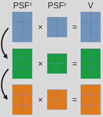
To quickly recap, the previous example involves calculating the total contribution, labeled as \(I\), from all molecules. These molecules are indexed by \(n\), and they relate to each pixel, which is indexed by \(i\) and \(j\). Referring to the assumptions discussed earlier, we can express the algorithm’s mathematical form as follows:

Now, shifting our focus to the present issue that involves multiple independent images (or frames), we extend the same calculation to each individual image, denoted as \(f\). As a result, the mathematical representation for this new problem takes the following shape (where $V$ stands for video):

The first implementation

Based on the description so far, we can readily enclose a for-loop iterating over \(f\) around the previously optimized code to create the initial version of our single-molecule video simulation code¹:

function video_sim_v1(xᵖ, yᵖ, x, y)
    F = size(x, 2)
    V = Array{eltype(x),3}(undef, length(xᵖ), length(yᵖ), F)
    for f in 1:F
        PSFˣ = exp.(-(xᵖ .- Transpose(view(x, :, f))) .^ 2)
        PSFʸ = exp.(-(view(y, :, f) .- Transpose(yᵖ)) .^ 2)
        V[:, :, f] = PSFˣ * PSFʸ
    end
    return V
end

Two points to note in the code above:

• x and y are both arrays of dimensions \(N\times F\), where \(N\) and \(F\) represent the number of molecule and number of frames, respectively.
• It appears that we have made a bold assumption that all frames contain an equal number of molecules. However, this assumption is acceptable since molecules that should not appear in a frame can be positioned far away from the field-of-view, thereby making no contribution.

Benchmarking video_sim_v1 using a dataset comprising 20 molecules and 100 frames (each with 256\(\times\)256 pixels) yields 50.927 ms (1402 allocations: 123.47 MiB). Our overarching goal entails improving upon this benchmark.

Optimization ideas

Before exploring new techniques, let’s take a moment to consider whether we can apply anything from my previous blog. Since we have only added one extra loop, there isn’t much opportunity to reduce memory allocation. What’s more, this extra loop cannot be easily eliminated through vectorization, as the formula specified here doesn’t align with basic matrix (or tensor) operations. Consequently, we must use other techniques to tackle this challenge.

In this video simulation problem, it is important to note that all frames are independent of each other. As a result, there is potential to simulate frames simultaneously, or in other words, in parallel.

Parallelism

Parallelizing an algorithm is much easier said than done. In view of the intricate nature of contemporary computational infrastructures, attaining parallelism in the present era involves three major tiers: core-level parallelism, node-level parallelism, and cluster-level parallelism². In the upcoming sections, I will delve into a single common scheme within each tier and examine its relevance within the context of our specific problem.

Core-level

This initial question that may arise is: how is it possible to achieve parallelism on a single core? To illustrate this, let’s consider a situation where a program operates on 64-bit integers, and a processor core possesses the capability to fetch 256 bits of data in a solitary operation. In such a scenario, it becomes viable to load four integers as a vector and perform a singular vectorized iteration of the original operation. This could potentially yield a theoretical speedup of fourfold³. This particular approach to parallelization is commonly known as “single instruction, multiple data” (SIMD).

The straightforward concept of SIMD, on one hand, allows numerous modern programming languages to identify points within an algorithm where SIMD can be employed and subsequently apply it automatically. On the other hand, SIMD is frequently constrained to basic operations such as addition or multiplication. Hence, the potential enhancement of video_sim_v1 through this method remains uncertain. Nevertheless, in this scenario, an attempt must be made to explore the possibilities.

In Julia, it is possible to enforce vectorization by employing the @simd macro, placed before a for-loop involving independent iterations. This technique results in the creation of video_sim_v2:

function video_sim_v2(xᵖ, yᵖ, x, y)
    F = size(x, 2)
    V = Array{eltype(x),3}(undef, length(xᵖ), length(yᵖ), F)
    @simd for f in 1:F
        PSFˣ = exp.(-(xᵖ .- Transpose(view(x, :, f))) .^ 2)
        PSFʸ = exp.(-(view(y, :, f) .- Transpose(yᵖ)) .^ 2)
        V[:, :, f] = PSFˣ * PSFʸ
    end
    return V
end

A benchmark analysis yields a result of 51.017 ms (1402 allocations: 123.47 MiB), indicating a lack of performance improvement. It seems that Julia has indeed automatically vectorized the code in this case.

Node-level

Moving up a level there is parallelism on a node (often a computer), which is often achieved through multithreading. For multithreading, we require multiple processors (either physical or virtual⁴), with each core being associated with a separate thread. Multithreading facilitates the simultaneous execution of these processors, all while utilizing the same memory pool. It is important to note that the implementation of multithreading demands careful consideration to avoid conflicts between threads. Fortunately, developers have often shouldered much of this responsibility, alleviating users of this burden.

In Julia, multithreading a for-loop can be as easy as follows⁵:

function video_sim_v3(xᵖ, yᵖ, x, y)
    F = size(x, 2)
    V = Array{eltype(x),3}(undef, length(xᵖ), length(yᵖ), F)
    Threads.@threads for f in 1:F
        PSFˣ = exp.(-(xᵖ .- Transpose(view(x, :, f))) .^ 2)
        PSFʸ = exp.(-(view(y, :, f) .- Transpose(yᵖ)) .^ 2)
        V[:, :, f] = PSFˣ * PSFʸ
    end
    return V
end

My desktop computer is equipped with four physical CPU cores, which translate into eight threads. When assessing the benchmark of video_sim_v3 with all eight threads, the results demonstrate a remarkable speedup of almost four times comparing to video_sim_v1, clocking in at 12.925 ms (1450 allocations: 123.47 MiB).

Cluster-level

Now assume you have access to a cluster, which is not uncommon for universities and institutes nowadays, you could even consider modifying the algorithm to execute across multiple processors spanning numerous computers. A frequently employed strategy involves the utilization of multiprocessing.

With the concept of multithreading in mind, we can easily comprehend multiprocessing as the simultaneous operation of multiple processors, where each core has access only to its designated memory space. This fundamental distinction from multithreading requires some “coding maneuvers” as users are now compelled to determine the allocation of data to individual processors. In the context of our example problem, implementing multiprocessing requires some rather major change of the code, contradicting the very impetus driving my blog posts. Therefore, I only provide a preliminary example in this GitHub repository of mine.

Key consideration

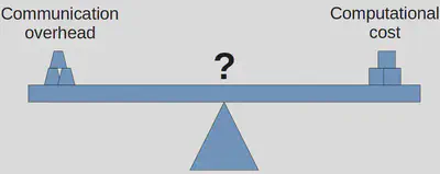
While I aimed to maintain a surface-level discourse in my blog, it is totally reasonable to feel confused when deciding upon a parallelization scheme. 😄 The crucial factor to bear in mind is that an escalation in the number of processors engaged directly corresponds to an increase in communication overhead. This rise in overhead can potentially overshadow the performance benefits gained from task distribution.

As of the post date of this blog, it is generally advisable to experiment with SIMD and multithreading in your code, as they are relatively easier to test. On the other hand, when it comes to multiprocessing, it is recommended to consider its implementation only when each discrete task consumes several seconds to execute, and the level of inter-process communication remains minimal.

Although it has been a long journey, our quest remains incomplete. There is one more concept, which is gaining popularity in recent years, that we can test. In the third part of my blog, I will discuss GPU computation.